

SITCOMTN-135
Pipeline Tasks in the AOS Wavefront Estimation Pipeline#
Abstract
Here we explain the Rubin Science Pipeline Tasks that make up the Active Optics System Wavefront Estimation Pipeline (WEP) and investigate timing and implementation of those tasks in a production environment.
WEP Pipeline Tasks#
The Wavefront Estimation Pipeline (WEP) is the code that will analyze defocal images and estimate the Rubin Observatory wavefront in terms of Zernike polynomials. The Rubin Active Optics System (AOS) will rely on these estimates to calculate the needed corrections to the optical system to maximize image quality. The pipeline runs as a set of Rubin Science Pipeline “Pipeline Tasks”. There are four sets of tasks that make up the pipeline of which the final three are developed by the Rubin AOS team and maintained on github in the ts_wep repository found at https://github.com/lsst-ts/ts_wep. The four jobs that the tasks perform are:
Instrument Signature Removal (ISR): This is performed on the raw images and the code for this task is developed by the Rubin DM team.
Catalog Generation
Postage Stamp Creation
Zernike Estimation
In this section we will describe the pipeline tasks that perform steps 2-4 in more detail.
Catalog Generation#
We have three main pipeline tasks that we can choose to use for catalog generation depending on our needs at the time.
Generate Catalogs From WCS and Reference Catalogs: We use the WCS supplied by the image and the reference catalogs available in the butler (e.g., Gaia) to run our source selection algorithms on catalog data and then identify the locations on the image with the WCS.
Generate Catalogs From Direct Detection: In the default mode for this task we convolve the image with a template defocused source (template donut created by raytracing code
batoid) and run source detection on the convolved image. We then run our source selection algorithms on the catalogs generated from this direct detection before saving a final set of sources to use for wavefront estimation. We anticipate that this mode will be most useful early in commissioning before an accurate pointing model is developed.Generate Catalogs From New WCS: When running with this task we combine the two tasks above. We run an initial source detection directly on the image and use these sources to fit a new WCS on the image. We then create a catalog using the new WCS and reference catalogs as in the first task above.
In each of these catalog generation steps we take the initial sources that exist on the image and run our own source selection algorithms to select only sources that will be appropriate for wavefront estimation. For more information on our source selection algorithms as well as deblending options see SITCOMTN-130.
Postage Stamp Creation#
This set of tasks all take in source catalogs generated by the previous catalog generation tasks and the post-ISR images and use them to cut out postage stamps of all the sources (defocal donuts) we want to use in wavefront estimation. When we load the post-ISR images we first perform background subtraction on the entire image before moving on to cut out postage stamps. This process occurs in two steps. We first cut out a larger section of the image around the source position given by the catalog. We then use a model template and convolve the stamp to recenter the stamp on the actual location of the source before cutting out a smaller postage stamp which is the size expected by the Zernike wavefront estimation task that follows. The recentering occurs because the actual location on the image for the source may be different than the catalog value especially if it was generated using the WCS and reference catalog. If this difference is too large we have a configuration that sets a maximum recentering distance and the recentering will not occur. The final stamp will be cut out in the original location and the stamp will be flagged in the task metadata as well as adding a warning message to the task log.
There are two separate tasks that perform the cut out step and they are different because of the properties of the specific wavefront sensors on the LSST Camera versus the science sensors on LSSTCam. The wavefront estimation currently implemented by the WEP requires pairs of intra-focal and extra-focal images to calculate the wavefront using the Transport of Intensity equation (TIE). The wavefront sensors on the LSST camera are offset from the science sensors by 1.5 mm with 4 half chips each in the extra-focal and intra-focal direction. Therefore, when using the wavefront sensors on LSSTCam all of the extra-focal and intra-focal images are taken in the same visit so we run the full WEP on images from a single exposure. When we are running AOS during commissioning with the LSST Commissioning Camera (ComCam) or the science sensors on LSSTCam we will need to piston the camera away from focus in one direction and take an exposure before pistoning to the opposite side of focus and taking another exposure. This requires storing the postage stamps cut out from pairs of visits together when running the WEP since the Zernike estimation works on pairs of intra-focal and extra-focal images. As a result when running WEP on science sensors we use a donut visit pair table to specify which exposures should have stamps grouped under the same data ID (we use the visit ID for the extra-focal visit) in the butler. The pair table can be generated in three different ways:
Manual: Users can generate their own pair tables specifying which intra-focal exposures and which extra-focal exposures should be grouped together. They can then ingest the table into the butler themselves for use with the pipeline.
Exposure Visit Info: This method uses information stored in the
visitInfothat accompanies each exposure in the butler and attempts to pair images automatically by finding images close in time, rotation and pointing location on the sky.Group ID: When taking the exposures we can specify a
GROUPIDvalue for each image that will be stored in the headers and propogate into the dimensions that can be queried by the butler. This method groups exposures with the same group ID value together.
Zernike Estimation#
Once the postage stamps are created and stored in the butler the final pipeline task that runs is the CalcZernikesTask. This task estimates the wavefront of the optical system using pairs of donuts. It does this for every pair of donuts on all sensors before averaging across each sensor. When running on science sensors where we piston the camera from one side of focus to the other while imaging the same field we match the same donut in the extra-focal image and intra-focal image. When running on wavefront sensors we have different areas of the sky falling on the extra-focal and intra-focal halves of each wavefront sensor. Therefore, when creating the pairs we cannot pair up two images of the same source. In this case we rank all the sources by brightness and then go down the ranked catalog pairing up the brightest extra-focal and intra-focal donut and then the second brightest in each half-sensor and so on. We continue down the ranked lists until we reach a specified number of sources or run out of sources on one of the halves of the sensor. Once we have the paired postage stamp images prepared we run the Zernike estimation. We currently have two methods implemented for Zernike estimation and two averaging methods. The two methods for calculating the Zernike estimates of the wavefront are:
Transport of Intensity Equation (TIE): This method uses the pairs of defocal sources on either side of focus to estimate the wavefront. For more information on this algorithm and how it is implemented in the WEP code see https://sitcomtn-111.lsst.io/.
Forward Modelling with Danish: This method uses the defocal image forward modelling code
danishto estimate the wavefront that produced the image and then expresses that in terms of Zernike polynomial coefficients. This method does not actually require pairs of images and implementing single side-of-focus results is something we will discuss in future work.
Once there are Zernike coefficients for each pair of sources we then must combine the results from all sources on each detector into a single value per detector to feed into the next step of the AOS code that actually uses the estimated wavefront to calculate the corrections to the optical system. To do this combination we have two methods:
combineZernikesMeanTask: This subtask just takes the mean of each Zernike coefficients across all sources on a detector.combineZernikesSigmaClipTask: This subtask uses sigma clipping of Zernike coefficients to remove outliers from the final mean.
At the end of this task each detector has a single array containing an averaged estimate of the wavefront in terms of Zernike polynomials that is stored in the butler.
Future Work#
While we are focused on preparing the pipeline we have already developed for testing during commissioning we do have some additional tasks we would like to add and test.
Single Side-of-Focus Zernike Estimation: The forward modeling method we currently have implemented with
danishallows us to estimate Zernikes from single donuts without the need for a pair. We need to do some code refactoring to enable this to work in the pipeline using data from single donuts.Machine Learning Zernike Estimation: We have a third Zernike estimation method based upon machine learning that directly estimates the Zernike coefficients from single donut images. For more information see Crenshaw et al. (2024).
Additional Resources#
Jupyter Notebooks#
The AOS team has additional documentation on the tasks including additional information on the configuration parameters available in a set of documentation notebooks in the ts_analysis_notebooks repository.
Here are some specific notebooks for each set of tasks:
Catalog Generation:
wepSourceSelectionWithWcs.ipynb: Explains more about generating donut catalogs with WCS and the reference catalogs.
Postage Stamp Creation:
cutOutDonutsWithWEP.ipynb: Shows how to run the donut cut out task interactively.
Zernike Estimation:
calcZernikesFromDonutStamps.ipynb: Demonstrates how to use the donut stamps stored in the butler to run the Zernike estimation pipeline task. Also includes additional details on the sigma clipping method to combine Zernike coefficients in the final output.
Code Documentation#
The WEP APIs and code structure are also extensively documented in the offical ts_wep repository documentation found at https://ts-wep.lsst.io/.
WEP Timing#
Running as a pipeline from command line#
The Active Optics System (AOS) will need to run completely between exposures during Rubin Observatory commissioning. With a realistic estimation of 3 seconds of overhead between exposures this gives us a time constraint of approximately 33 seconds to run the complete AOS including propogating corrections through to the optical system. Therefore, the WEP needs to run in 25-30 seconds to leave time for the corrections to be made.
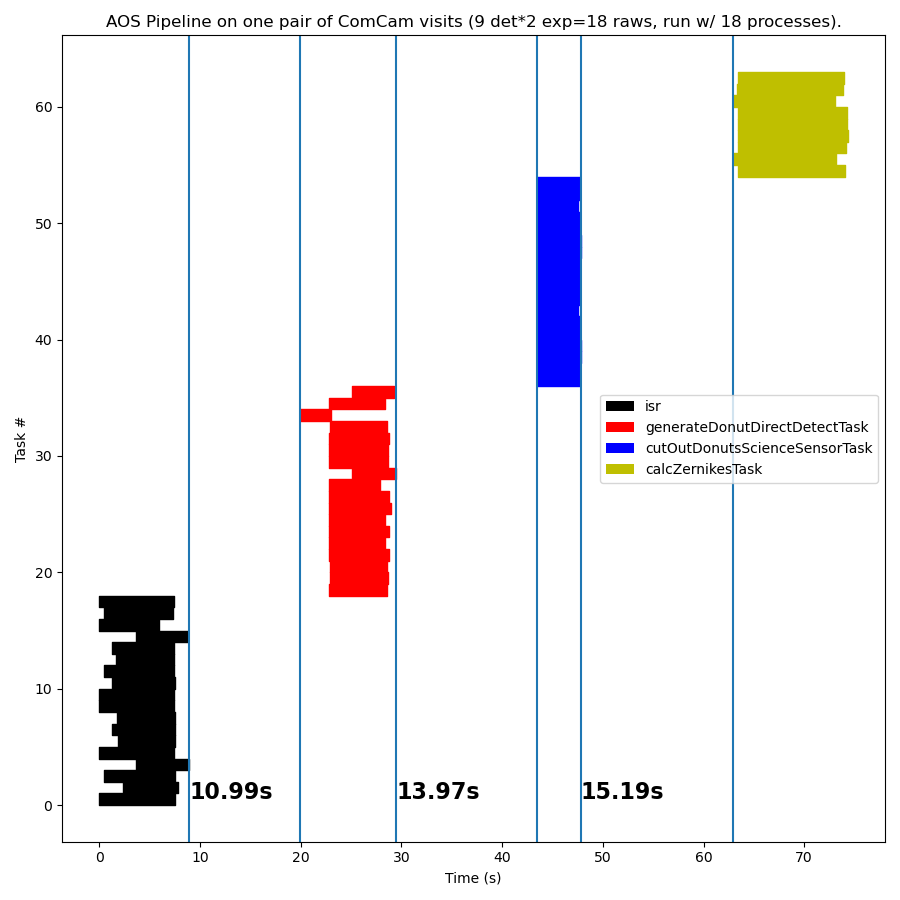
Using version 10.4 of ts_wep on the USDF we ran the pipeline using the slurm scheduler running the WEP from the command line using the pipetask run command on one pair of simulated ComCam visits. We have included the slurm scripts and pipeline configuration as well as a notebook analyzing the results to make the plots in this section in the notebooks folder accompanying this technote. With ComCam we need a pair of visits so there are 18 total exposures. We ran with 18 processes so that we would have enough at each step of the pipeline and we limited the number of sources in the catalog for each detector to 5. Figure 1 below shows the results with the bold numbers showing the time between different tasks ending and the subsequent set of tasks starting. We see that the total time for the pipeline is about 75 seconds but approximately 40 seconds is taken up by empty time between sets of tasks.
Upon seeing the gaps between tasks we contacted Rubin Data Management for input with the following JIRA ticket: DM-45524. It was suggested that the gaps are due to startup time between each new process as the processes that complete one set of task finish they are killed and new ones must load python and data to accomplish the next set of tasks. The very long time gaps are a result of the slow /sdf filesystem on USDF. When Andy Salnikov ran on lscratch on USDF, the fast local disk on one of the USDF machines we found the following shown in Figure 2.
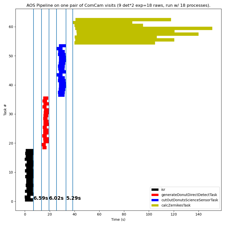
This test ran using the full donut catalogs so the timing of the final Zernike estimation step is much longer but the difference we are interested in is the time between sets of tasks. Using the fast, local filesystem we see that the time gaps are cut by more than half to a total to 18 seconds. If we had only used 5 sources so that we had the same time in tasks as the first test this would give us a full pipeline run time of about 53 seconds. This time is closer to our goal of 25 seconds but still about half a minute off. Looking at Figure 2 we see that there are still two areas where we are losing significant time that is solely related to multiprocessing and the filesystem. The first is that there are still 18 seconds of time gaps between running sets of tasks. The second is that there is variability in the start time for all the processes running the same type of task that costs us an additional 5-10 seconds. Solving these two issues together would likely be enough to run the pipeline in the time needed with 5 sources on each detector. Luckily the WEP will not run from the command line in commissioning be will be a part of the Rapid Analysis (RA) tooling which we will explain in the next section.
Running inside Rapid Analysis#
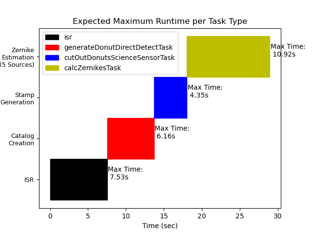
The Rapid Analysis (RA) code is a framework running on Kubernetes pods at the summit (and other places) to perform realtime processing on the latest images as they are taken. More details on RA can be found in SITCOMTN-100 which is a technote in development describing RA and Rubin TV. One of the major advantages of the RA system is that it will always have processses available within the Kubernetes pods to run analysis without needing the reload and import time we saw on the USDF filesystem. Since AOS will be one of the main customers of RA we have been working with the primary RA developer Merlin Fisher-Levine to integrate the WEP pipeline as much as possible into RA. At this moment ISR which is a common task for multiple RA customers in integrated into the main Single Frame Measurement (SFM) pipeline within RA. In addition, we have worked with Merlin so that the Catalog Creation step will also be run as part of the SFM pipeline when RA detects that an AOS related image arrives. That leaves the final two steps in the pipeline as a separate smaller AOS pipeline that will run within RA when AOS images arrive from the camera. We are also adding additional plotting tasks that will create plots for Rubin TV that will run alongside these main WEP tasks. In Figure 3 we use the maximum time taken in the previous tests for an individual process to run each of the WEP tasks to generate a worst case scenario for each task. We then stack them together without time gaps to give us an approximate time to run the full WEP within RA. The figure shows that running WEP in Rapid Analysis with 5 sources per detector allows to run the full pipeline at around 29 seconds which meets our goal of 25-30 seconds for commissioning. We will soon run tests to see how this expected run time compares to what we actually get once everything is integrated into RA.
Future Work#
The current expected run time of 29 seconds within RA means that we expect to be able to run AOS as we start commissioning we would like to continue to optimize the time the WEP takes to make it more robust. Additional time allows us to look at additional sources when running Zernike estimation which helps makes our estimates more robust to outliers. In addition, we will need to see how long the Optical Feedback Controller system takes to get the estimated wavefront from the butler repository and calculate corrections and then administer those corrections within the optical system. Future areas of work we are looking at to improve the speed of the WEP are:
Machine Learning: Crenshaw et al. (2024) describes the development of machine learning techniques to perform Zernike estimation on defocal images from the Rubin Observatory. We plan on implementing and testing this during commissioning. The current deep learning model runs 40 times faster than the baseline TIE algorithm when estimating Zernikes which could give us many more sources while still reducing the time the Zernike estimation task takes.
Single Side of Focus Zernike Estimation: We are working on implementing code to enable the TIE and
danishto run within the WEP using only defocal sources from a single side of focus. Being able to run in this mode would allow us to run the full pipeline on just extra-focal or intra-focal images so that we could perform Zernike estimation on each side of focus when pistioning the camera during full focal plane AOS studies rather than waiting for the images from both sides of focus to be done before starting Zernike estimation. When running on wavefront sensors where a single image is taken this would give us twice as many sources that could be run at the same time.
Additional Resources#
Jupyter Notebooks#
The notebook used to make the plots in this section can be found along with other useful utility notebooks at ts_aos_analysis.
WEP Timing Notebook:
wep_pipeline_timing.ipynb: Analyze the timing of the WEP on the USDF.